Automatic Construction of Bootstrap Confidence Intervals

Introduction

Bootstrap confidence intervals depend on three elements:

the cdf of the $B$ bootstrap replications $t_i^*$ , $i=1\ldots B$
the bias-correction number $z_0 = \Phi(\sum_i^B I(t_i^* < t_0) / B )$ where $t_0=f(x)$ is the original estimate
the acceleration number $a$ that measures the rate of change in $\sigma_{t_0}$ as $x$ , the data changes.

The first two of these depend only on the bootstrap distribution, and not how it is generated: parametrically or non-parametrically.

Package bcaboot aims to make construction of bootstrap confidence intervals almost automatic. The two main functions are:

bca_nonpar() for nonparametric bootstrap
bca_par() for parametric bootstrap

All results are returned as bcaboot objects with a consistent structure and support tidy(), glance(), and autoplot() for integration with the tidyverse ecosystem.

Further details are in the Efron and Narasimhan (2020) paper. Much of the theory behind the approach can be found in references Efron (1987), T. DiCiccio and Efron (1992), T. J. DiCiccio and Efron (1996), and Efron and Hastie (2016).

A Nonparametric Example

Suppose we wish to construct bootstrap confidence intervals for an $R^2$ -statistic from a linear regression. Using the diabetes data from the lars (442 by 11) as an example, we use the function below to regress the y on x, a matrix of of 10 predictors, to compute $R^2$ .

data(diabetes, package = "bcaboot")
Xy <- cbind(diabetes$x, diabetes$y)
rfun <- function(Xy) {
    y <- Xy[, 11]
    X <- Xy[, 1:10]
    summary(lm(y ~ X) )$adj.r.squared
}

Constructing bootstrap confidence intervals involves merely calling bca_nonpar:

set.seed(1234)
result <- bca_nonpar(x = Xy, B = 2000, func = rfun, verbose = FALSE)

The result prints a clean summary:

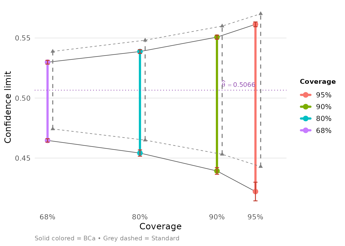
result

##  conf.level    bca.lo    bca.hi    std.lo    std.hi
##        0.95 0.4221740 0.5613841 0.4429423 0.5701783
##        0.90 0.4392968 0.5507219 0.4531704 0.5599503
##        0.80 0.4541906 0.5387434 0.4649627 0.5481579
##        0.68 0.4647324 0.5298461 0.4742814 0.5388392

Tidy output

The tidy() method returns a tibble with one row per (confidence level, method) combination, following the broom conventions:

tidy(result)

## # A tibble: 8 × 7
##   conf.level method   estimate conf.low conf.high jacksd.low jacksd.high
##        <dbl> <chr>       <dbl>    <dbl>     <dbl>      <dbl>       <dbl>
## 1       0.95 bca         0.507    0.422     0.561    0.00776     0.00201
## 2       0.95 standard    0.507    0.443     0.570   NA          NA      
## 3       0.9  bca         0.507    0.439     0.551    0.00280     0.00173
## 4       0.9  standard    0.507    0.453     0.560   NA          NA      
## 5       0.8  bca         0.507    0.454     0.539    0.00262     0.00157
## 6       0.8  standard    0.507    0.465     0.548   NA          NA      
## 7       0.68 bca         0.507    0.465     0.530    0.00143     0.00158
## 8       0.68 standard    0.507    0.474     0.539   NA          NA

The glance() method provides a one-row summary of the bootstrap run:

glance(result)

## # A tibble: 1 × 9
##   method accel      theta sdboot     z0        a sdjack     B boot_mean
##   <chr>  <chr>      <dbl>  <dbl>  <dbl>    <dbl>  <dbl> <dbl>     <dbl>
## 1 nonpar regression 0.507 0.0325 -0.268 -0.00585 0.0323  2000     0.515

Visualization

When ggplot2 is available, autoplot() produces a publication-ready plot of the confidence intervals:

library(ggplot2)
autoplot(result)

Acceleration methods

The accel argument controls how the acceleration $a$ is estimated:

accel = "regression" (default): uses local regression on bootstrap count vectors nearest to uniform. Also computes the gbca diagnostic.
accel = "jackknife": uses classical delete-one (or delete-group) jackknife influence values.

set.seed(1234)
result_jk <- bca_nonpar(x = Xy, B = 2000, func = rfun,
                        accel = "jackknife", verbose = FALSE)
tidy(result_jk)

## # A tibble: 8 × 7
##   conf.level method   estimate conf.low conf.high jacksd.low jacksd.high
##        <dbl> <chr>       <dbl>    <dbl>     <dbl>      <dbl>       <dbl>
## 1       0.95 bca         0.507    0.435     0.560    0.00412     0.00155
## 2       0.95 standard    0.507    0.443     0.570   NA          NA      
## 3       0.9  bca         0.507    0.443     0.551    0.00497     0.00224
## 4       0.9  standard    0.507    0.453     0.560   NA          NA      
## 5       0.8  bca         0.507    0.454     0.540    0.00127     0.00158
## 6       0.8  standard    0.507    0.465     0.548   NA          NA      
## 7       0.68 bca         0.507    0.464     0.531    0.00186     0.00177
## 8       0.68 standard    0.507    0.474     0.539   NA          NA

A Parametric Example

A logistic regression was fit to data on 812 neonates at a large clinic. Here is a summary of the dataset.

str(neonates)

## 'data.frame':    812 obs. of  12 variables:
##  $ gest: num  -0.729 -0.729 1.156 -2.884 0.348 ...
##  $ ap  : num  0.856 0.856 0.856 -2.076 0.856 ...
##  $ bwei: num  -0.694 -0.694 0.786 -2.174 0.786 ...
##  $ gen : num  1.227 -0.814 -0.814 1.227 -0.814 ...
##  $ resp: num  0.78 -0.939 1.639 1.639 1.639 ...
##  $ head: num  -0.402 -0.402 -0.402 -0.402 -0.402 ...
##  $ hr  : num  -0.256 -0.256 -0.256 -0.256 -0.256 ...
##  $ cpap: num  1.866 -0.535 1.866 1.866 1.866 ...
##  $ age : num  -0.94 -0.94 -0.94 -0.94 1.06 ...
##  $ temp: num  -0.669 -0.669 -0.669 -0.669 2.339 ...
##  $ size: num  0.484 -1.319 -1.319 0.484 0.484 ...
##  $ y   : int  1 1 1 1 1 1 1 1 1 1 ...

The goal was to predict death versus survival— $y$ is 1 or 0, respectively—on the basis of 11 baseline variables of which one of them resp was of particular concern. (There were 207 deaths and 605 survivors.) So here $\theta$ , the parameter of interest is the coefficient of resp. Discussions with the investigator suggested a weighting of 4 to 1 of deaths versus non-deaths.

A Logistic Model

weights <- with(neonates, ifelse(y == 0, 1, 4))
glm_model <- glm(formula = y ~ ., family = "binomial", weights = weights, data = neonates)
summary(glm_model)

## 
## Call:
## glm(formula = y ~ ., family = "binomial", data = neonates, weights = weights)
## 
## Coefficients:
##             Estimate Std. Error z value Pr(>|z|)    
## (Intercept) -0.26510    0.07598  -3.489 0.000485 ***
## gest        -0.70602    0.13117  -5.383 7.35e-08 ***
## ap          -0.78594    0.07874  -9.982  < 2e-16 ***
## bwei        -0.23332    0.12592  -1.853 0.063879 .  
## gen         -0.04107    0.07355  -0.558 0.576594    
## resp         0.94306    0.08974  10.509  < 2e-16 ***
## head         0.04813    0.08057   0.597 0.550299    
## hr           0.03504    0.07191   0.487 0.626045    
## cpap         0.43438    0.08869   4.898 9.70e-07 ***
## age          0.15727    0.08492   1.852 0.064041 .  
## temp        -0.05960    0.08506  -0.701 0.483520    
## size        -0.37477    0.09919  -3.778 0.000158 ***
## ---
## Signif. codes:  0 '***' 0.001 '**' 0.01 '*' 0.05 '.' 0.1 ' ' 1
## 
## (Dispersion parameter for binomial family taken to be 1)
## 
##     Null deviance: 1951.7  on 811  degrees of freedom
## Residual deviance: 1187.2  on 800  degrees of freedom
## AIC: 1211.2
## 
## Number of Fisher Scoring iterations: 5

Parametric bootstrapping in this context requires us to independently sample the response according to the estimated probabilities from regression model. As discussed in the paper accompanying this software, routine bca_par also requires sufficient statistics $\hat{\beta} = M^\prime y$ where $M$ is the model matrix. Therefore, it makes sense to have a function do the work. The function glm_boot below returns a list of the estimate $\hat{\theta}$ , the bootstrap estimates, and the sufficient statistics.

glm_boot <- function(B, glm_model, weights, var = "resp") {
    pi_hat <- glm_model$fitted.values
    n <- length(pi_hat)
    y_star <- sapply(seq_len(B), function(i) ifelse(runif(n) <= pi_hat, 1, 0))
    beta_star <- apply(y_star, 2, function(y) {
        boot_data <- glm_model$data
        boot_data$y <- y
        coef(glm(formula = y ~ ., data = boot_data, weights = weights, family = "binomial"))
    })
    list(theta = coef(glm_model)[var],
         theta_star = beta_star[var, ],
         suff_stat = t(y_star) %*% model.matrix(glm_model))
}

Now we can compute the bootstrap estimates using bca_par.

set.seed(3891)
glm_boot_out <- glm_boot(B = 2000, glm_model = glm_model, weights = weights)
glm_bca <- bca_par(t0 = glm_boot_out$theta,
                   tt = glm_boot_out$theta_star,
                   bb = glm_boot_out$suff_stat)

We can examine the results using tidy methods:

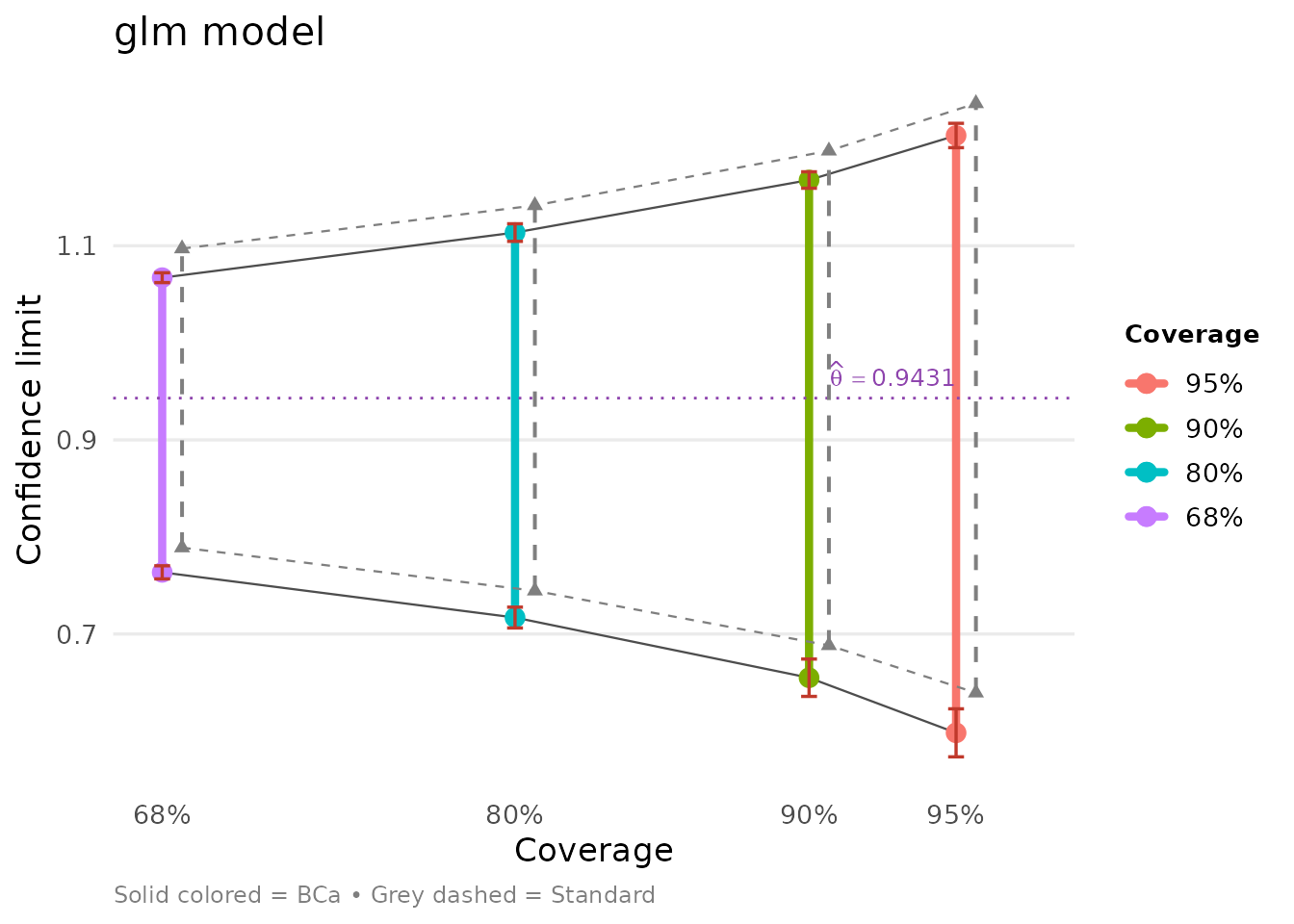
glm_bca

##  conf.level    bca.lo   bca.hi    std.lo   std.hi
##        0.95 0.5981733 1.213676 0.6394385 1.246691
##        0.90 0.6549470 1.167789 0.6882535 1.197876
##        0.80 0.7169529 1.113660 0.7445341 1.141595
##        0.68 0.7635391 1.067160 0.7890090 1.097120

tidy(glm_bca)

## # A tibble: 8 × 7
##   conf.level method   estimate conf.low conf.high jacksd.low jacksd.high
##        <dbl> <chr>       <dbl>    <dbl>     <dbl>      <dbl>       <dbl>
## 1       0.95 bca         0.943    0.598      1.21    0.0247      0.0125 
## 2       0.95 standard    0.943    0.639      1.25   NA          NA      
## 3       0.9  bca         0.943    0.655      1.17    0.0193      0.00848
## 4       0.9  standard    0.943    0.688      1.20   NA          NA      
## 5       0.8  bca         0.943    0.717      1.11    0.0107      0.00907
## 6       0.8  standard    0.943    0.745      1.14   NA          NA      
## 7       0.68 bca         0.943    0.764      1.07    0.00676     0.00507
## 8       0.68 standard    0.943    0.789      1.10   NA          NA

Our bootstrap standard error using $B=2000$ samples for resp can be read off from the glance output:

glance(glm_bca)

## # A tibble: 1 × 9
##   method accel theta sdboot     z0       a sdjack     B boot_mean
##   <chr>  <chr> <dbl>  <dbl>  <dbl>   <dbl>  <dbl> <dbl>     <dbl>
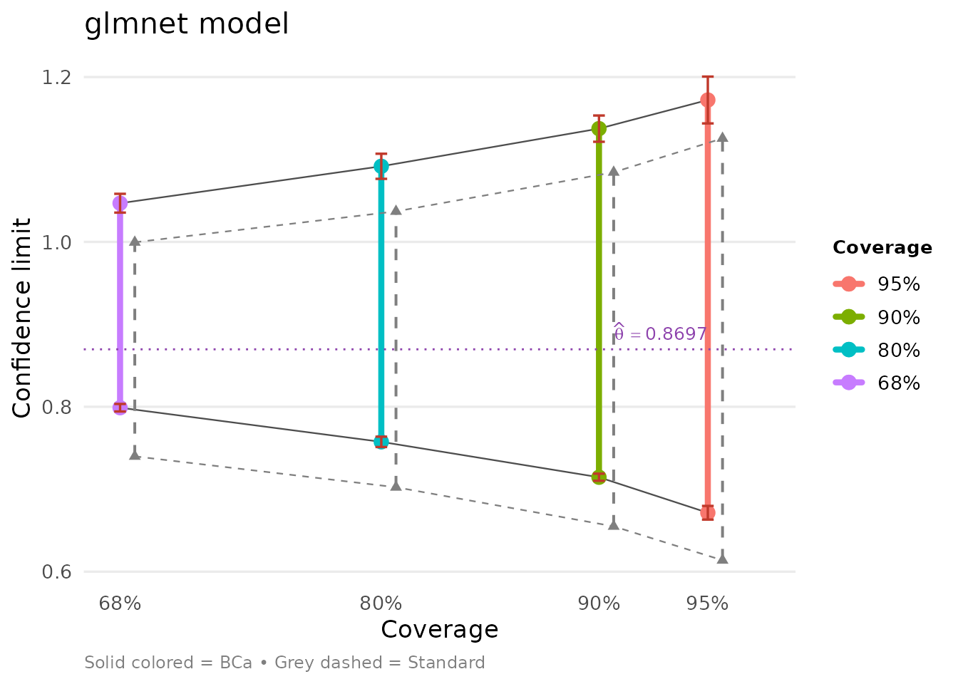
## 1 par    NA    0.943  0.155 -0.215 -0.0194     NA  2000     0.982

A Penalized Logistic Model

Now suppose we wish to use a nonstandard estimation procedure, for example, via the glmnet package, which uses cross-validation to figure out a best fit, corresponding to a penalization parameter $\lambda$ (named lambda.min).

X <- as.matrix(neonates[, seq_len(11)]) ; Y <- neonates$y;
glmnet_model <- glmnet::cv.glmnet(x = X, y = Y, family = "binomial", weights = weights)

We can examine the estimates at the lambda.min as follows.

coefs <- as.matrix(coef(glmnet_model, s = glmnet_model$lambda.min))
knitr::kable(data.frame(variable = rownames(coefs), coefficient = coefs[, 1]), row.names = FALSE, digits = 3)

variable	coefficient
(Intercept)	-0.212
gest	-0.540
ap	-0.687
bwei	-0.268
gen	0.000
resp	0.870
head	0.000
hr	0.000
cpap	0.382
age	0.050
temp	0.000
size	-0.221

Following the lines above, we create a helper function to perform the bootstrap.

glmnet_boot <- function(B, X, y, glmnet_model, weights, var = "resp") {
    lambda <- glmnet_model$lambda.min
    theta <- as.matrix(coef(glmnet_model, s = lambda))
    pi_hat <- predict(glmnet_model, newx = X, s = "lambda.min", type = "response")
    n <- length(pi_hat)
    y_star <- sapply(seq_len(B), function(i) ifelse(runif(n) <= pi_hat, 1, 0))
    beta_star <- apply(y_star, 2,
                       function(y) {
                           as.matrix(coef(glmnet::glmnet(x = X, y = y, lambda = lambda, weights = weights, family = "binomial")))
                       })

    rownames(beta_star) <- rownames(theta)
    list(theta = theta[var, ],
         theta_star = beta_star[var, ],
         suff_stat = t(y_star) %*% X)
}

And off we go.

glmnet_boot_out <- glmnet_boot(B = 2000, X, y, glmnet_model, weights)
glmnet_bca <- bca_par(t0 = glmnet_boot_out$theta,
                      tt = glmnet_boot_out$theta_star,
                      bb = glmnet_boot_out$suff_stat)

We can compare both models side-by-side:

autoplot(glm_bca) + ggtitle("glm model")

autoplot(glmnet_bca) + ggtitle("glmnet model")

Ratio of Independent Variance Estimates

Assume we have two independent estimates of variance from normal theory:

$\hat{\sigma}_1^2\sim\frac{\sigma_1^2\chi_{n_1}^2}{n_1},$

and

$\hat{\sigma}_2^2\sim\frac{\sigma_2^2\chi_{n_2}^2}{n_2}.$

Suppose now that our parameter of interest is

$\theta=\frac{\sigma_1^2}{\sigma_2^2}$

for which we wish to compute confidence limits. In this setting, theory yields exact limits:

$\hat{\theta}(\alpha) = \frac{\hat{\theta}}{F_{n_1,n_2}^{1-\alpha}}.$

We can apply bca_par to this problem. As before, here are our helper functions.

ratio_boot <- function(B, v1, v2) {
    s1 <- sqrt(v1) * rchisq(n = B, df = n1)  / n1
    s2 <- sqrt(v2) * rchisq(n = B, df = n2)  / n2
    theta_star <- s1 / s2
    beta_star <- cbind(s1, s2)
    list(theta = v1 / v2,
         theta_star = theta_star,
         suff_stat = beta_star)
}

funcF <- function(beta) {
    beta[1] / beta[2]
}

Note that we have an additional function funcF which corresponds to $\tau(\hat{\beta}^*)$ in the paper. This is the function expressing the parameter of interest as a function of the sample.

B <- 16000; n1 <- 10; n2 <- 42
ratio_boot_out <- ratio_boot(B, 1, 1)
ratio_bca <- bca_par(t0 = ratio_boot_out$theta,
                     tt = ratio_boot_out$theta_star,
                     bb = ratio_boot_out$suff_stat, func = funcF)

The tidy output shows the BCa, standard, and ABC limits:

tidy(ratio_bca)

## # A tibble: 12 × 7
##    conf.level method   estimate conf.low conf.high jacksd.low jacksd.high
##         <dbl> <chr>       <dbl>    <dbl>     <dbl>      <dbl>       <dbl>
##  1       0.95 abc             1   0.405       3.42   NA           NA     
##  2       0.95 bca             1   0.412       3.14    0.00824      0.0957
##  3       0.95 standard        1  -0.0527      2.05   NA           NA     
##  4       0.9  abc             1   0.472       2.73   NA           NA     
##  5       0.9  bca             1   0.475       2.57    0.00743      0.0426
##  6       0.9  standard        1   0.117       1.88   NA           NA     
##  7       0.8  abc             1   0.562       2.15   NA           NA     
##  8       0.8  bca             1   0.559       2.09    0.00687      0.0316
##  9       0.8  standard        1   0.312       1.69   NA           NA     
## 10       0.68 abc             1   0.646       1.81   NA           NA     
## 11       0.68 bca             1   0.639       1.77    0.00635      0.0247
## 12       0.68 standard        1   0.466       1.53   NA           NA

We can compare against exact F-distribution limits:

exact <- 1 / qf(df1 = n1, df2 = n2, p = 1 - as.numeric(rownames(ratio_bca$limits)))
knitr::kable(cbind(ratio_bca$limits, exact = exact), digits = 3)

	bca	jacksd	std	pct	exact
0.025	0.412	0.008	-0.053	0.068	0.422
0.05	0.475	0.007	0.117	0.104	0.484
0.1	0.559	0.007	0.312	0.164	0.570
0.16	0.639	0.006	0.466	0.228	0.650
0.5	1.046	0.006	1.000	0.570	1.053
0.84	1.772	0.025	1.534	0.903	1.800
0.9	2.095	0.032	1.688	0.953	2.128
0.95	2.573	0.043	1.883	0.985	2.655
0.975	3.141	0.096	2.053	0.996	3.247

Clearly the BCa limits match the exact values very well and suggests a large upward correction to the standard limits.

autoplot(ratio_bca)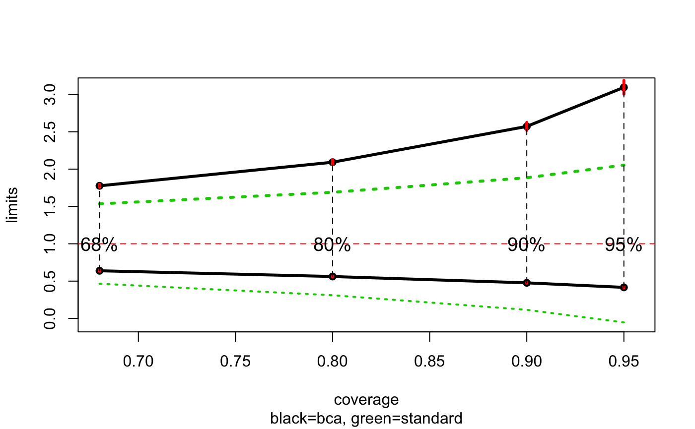

Migration from pre-1.0 API

Version 1.0 introduces a new API. The old functions continue to work but emit deprecation warnings. Here is how to migrate:

Function mapping

Old function	New function	Notes
`bcajack(x, B, func)`	`bca_nonpar(x, B, func, accel = "jackknife")`	Classical jackknife acceleration
`bcajack2(x, B, func)`	`bca_nonpar(x, B, func, accel = "regression")`	Regression acceleration (default)
`bcanon(B, x, func)`	`bca_nonpar(x, B, func)`	Removed; note argument order change
`bcapar(t0, tt, bb)`	`bca_par(t0, tt, bb)`
`bcaplot(result)`	`autoplot(result)`	Requires ggplot2

Parameter mapping

Old	New	Description
`alpha`	`conf.level`	E.g., `alpha = 0.025` becomes `conf.level = 0.95`
`m`	`n_groups`	Number of jackknife groups
`mr`	`group_reps`	Random grouping repetitions
`pct`	`kl_fraction`	Fraction of nearby count vectors
`K`	`n_jack`	Delete-d jackknife repetitions
`J`	`jack_groups`	Groups per jackknife fold
`trun`	`truncation`	Truncation for acceleration
`cd`	`conf_density`	Confidence density flag
`B` (as list)	`boot_data`	Pre-computed bootstrap data

Return structure

The new objects use $limits (not $lims), $B_mean (not $B.mean), and $stats is always a 2-row matrix (never a named vector). Use tidy() and glance() instead of accessing list components directly:

## Old way
result$lims[, "bca"]
result$stats["theta"]

## New way
tidy(result)    # tibble of confidence limits
glance(result)  # tibble of summary statistics

Deprecation timeline

Release	Status
1.0	Old functions work with once-per-session warning
1.1	Old functions error with migration message
2.0	Old functions removed

References

DiCiccio, Thomas J., and Bradley Efron. 1996. “Bootstrap Confidence Intervals.” Statist. Sci. 11 (3): 189–228. https://doi.org/10.1214/ss/1032280214.

DiCiccio, Thomas, and Bradley Efron. 1992. “More Accurate Confidence Intervals in Exponential Families.” Biometrika 79 (2): 231–45. https://doi.org/10.2307/2336835.

Efron, Bradley. 1987. “Better Bootstrap Confidence Intervals.” Journal of the American Statistical Association 82 (397): 171–85. https://doi.org/10.2307/2289144.

Efron, Bradley, and Trevor Hastie. 2016. Computer Age Statistical Inference: Algorithms, Evidence, and Data Science. 1st ed. New York, NY, USA: Cambridge University Press.

Efron, Bradley, and Balasubramanian Narasimhan. 2020. “The Automatic Construction of Bootstrap Confidence Intervals.” Journal of Computational and Graphical Statistics 29 (3): 608–19. https://doi.org/10.1080/10618600.2020.1714633.

Bradley Efron and Balasubramanian Narasimhan

2026-04-08