6 Changing the Loss: Huber, Quantile, LAD

What you’ll be able to do

Swap a squared-error loss for a Huber (robust) or quantile (asymmetric) loss by editing a single line, and understand how each changes the estimator.

6.1 The loss is a knob

Every regression in this book has the shape

\[\underset{\beta}{\mbox{minimize}}\quad \sum_i \phi\big(y_i - x_i^\top\beta\big),\]

and the choice of the loss \(\phi\) is the choice of estimator. Squared loss gives least squares. In Chapter 2 we already swapped it for absolute value (\(\phi(u)=|u|\)) to get least-absolute-deviation regression — one edited line. This chapter takes that idea seriously: two more losses, two more estimators, same code.

6.2 Huber: robust to outliers

Least squares is famously sensitive to outliers — a few bad points drag the whole fit. The Huber loss behaves like squared error for small residuals but only linearly for large ones, so outliers pull less:

\[ \phi_M(u) = \begin{cases} u^2 & |u| \le M \\ 2M|u| - M^2 & |u| > M. \end{cases} \]

To see it, we generate a one-predictor problem and flip the sign of 10% of the responses — nasty outliers by construction.

set.seed(1289)
m <- 450; M <- 1; pflip <- 0.10
beta_true <- 5
X <- matrix(rnorm(m), ncol = 1)
y_true <- X * beta_true
flip <- 2 * rbinom(m, 1, 1 - pflip) - 1     # -1 flips the sign
y <- flip * y_true + rnorm(m)

Now fit the same problem with two losses — squared and Huber:

beta <- Variable(1)

ols <- Problem(Minimize(sum_squares(y - X %*% beta)))
psolve(ols); beta_ols <- value(beta)

[1] 4494.614

hub <- Problem(Minimize(sum(huber(y - X %*% beta, M))))
psolve(hub); beta_hub <- value(beta)

[1] 1046.055

c(true = beta_true, OLS = beta_ols, Huber = beta_hub)

    true      OLS    Huber 
5.000000 4.160588 4.966967

The Huber estimate sits far closer to the truth (5); OLS is dragged toward zero by the flipped points. Only the loss line changed.

ggplot(data.frame(X = X, y = y), aes(X, y)) +
  geom_point(alpha = 0.3) +
  geom_abline(aes(slope = beta_ols,  intercept = 0, color = "OLS"),   linewidth = 1) +
  geom_abline(aes(slope = beta_hub,  intercept = 0, color = "Huber"), linewidth = 1) +
  geom_abline(aes(slope = beta_true, intercept = 0, color = "Truth"),
              linetype = "dashed") +
  scale_color_manual(values = c(OLS = "red", Huber = "blue", Truth = "black"),
                     name = NULL) +
  theme_minimal()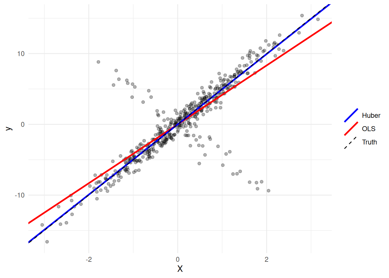

OLS is pulled toward the outliers; Huber resists.

6.3 Quantile: an asymmetric loss

Least squares estimates the conditional mean. To estimate a conditional quantile — say the 10th or 90th percentile — we tilt the absolute-value loss so that over- and under-prediction are penalized unequally:

\[\phi_\tau(u) = \tfrac{1}{2}|u| + \big(\tau - \tfrac{1}{2}\big)u, \qquad \tau \in (0,1).\]

At \(\tau = 0.5\) this is symmetric (the median / LAD); push \(\tau\) up or down and the fit tracks a higher or lower quantile. In CVXR it is, again, a one-line function:

quant_loss <- function(u, tau) 0.5 * abs(u) + (tau - 0.5) * u

We make data whose spread grows with \(x\) (heteroscedastic), so different quantiles fan out:

set.seed(7)
nq <- 200
xq <- runif(nq, 0, 4)
yq <- 1 + 2 * xq + rnorm(nq, sd = 0.5 + xq)   # noise widens with x
Xq <- cbind(1, xq)

Fit several quantiles — the same solve, only tau changes:

taus <- c(0.1, 0.5, 0.9)
bq <- Variable(2)
coefs <- sapply(taus, function(tau) {
  prob <- Problem(Minimize(sum(quant_loss(yq - Xq %*% bq, tau))))
  psolve(prob, solver = "CLARABEL")   # robust choice for the kink at tau = 0.5
  check_solver_status(prob)
  value(bq)
})
colnames(coefs) <- paste0("tau=", taus)
round(coefs, 3)

     tau=0.1 tau=0.5 tau=0.9
[1,]  -0.147   1.399   1.437
[2,]   1.001   1.889   3.453

df_lines <- data.frame(tau = factor(taus),
                       intercept = coefs[1, ], slope = coefs[2, ])
ggplot(data.frame(xq, yq), aes(xq, yq)) +
  geom_point(alpha = 0.3) +
  geom_abline(data = df_lines,
              aes(intercept = intercept, slope = slope, color = tau),
              linewidth = 1) +
  labs(x = "x", y = "y", color = expression(tau)) +
  theme_minimal()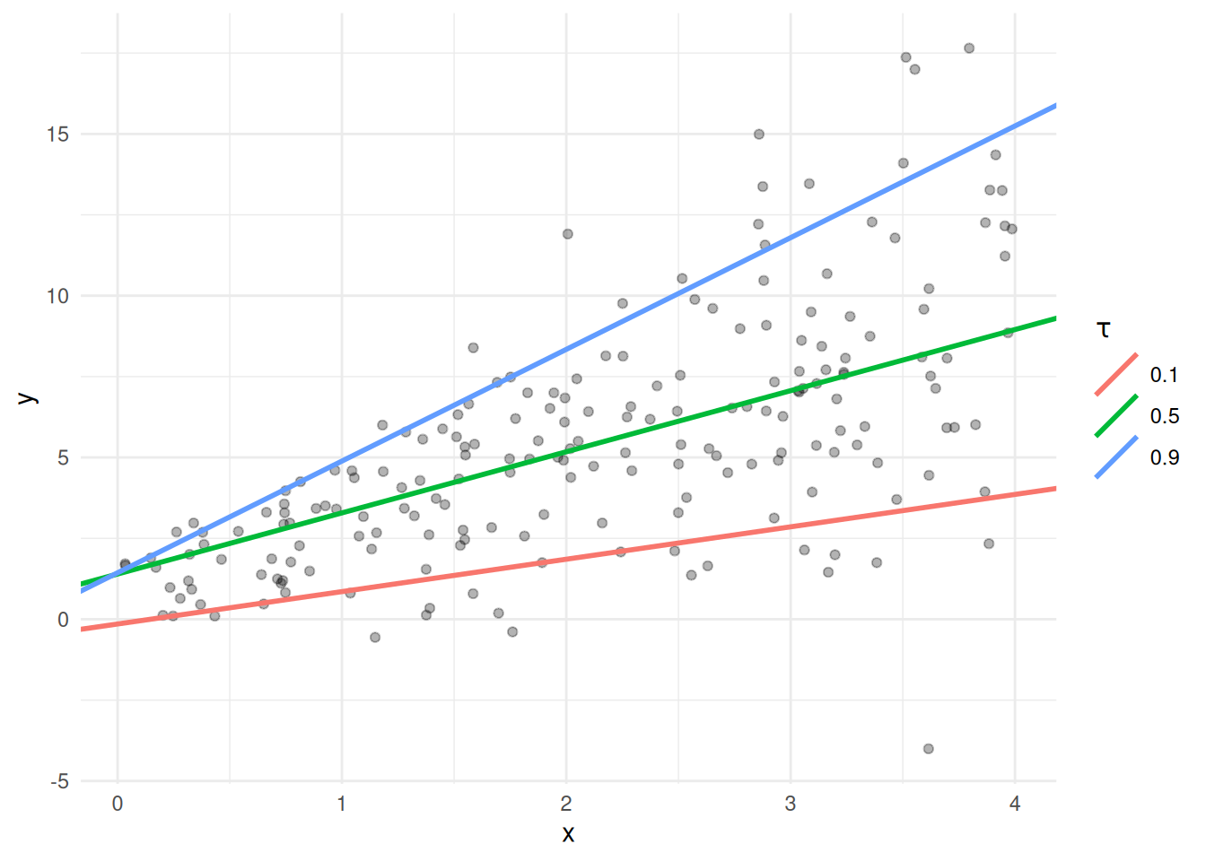

Quantile fits fan out where the spread is largest.

The three lines spread apart as \(x\) (and the noise) grows — exactly what quantile regression is for.

6.4 Exercise

Exercise (⭐). The Huber threshold \(M\) interpolates between two losses. What does Huber regression become as \(M \to 0\)? As \(M \to \infty\)? Check the small-\(M\) case against the LAD fit from Chapter 2.

Solution

As \(M \to 0\) the quadratic region vanishes and Huber \(\to\) (a scaled) absolute loss — LAD regression. As \(M \to \infty\) everything is “small,” so Huber \(\to\) squared loss — OLS.

small_M <- Problem(Minimize(sum(huber(y - X %*% beta, 0.01))))
psolve(small_M); val_small <- value(beta)

[1] 14.00813

lad <- Problem(Minimize(sum(abs(y - X %*% beta))))
psolve(lad); val_lad <- value(beta)

[1] 702.6453

c(huber_smallM = val_small, LAD = val_lad)

huber_smallM          LAD 
    5.028715     5.031708

The two nearly coincide.

6.5 Takeaways

The loss is the estimator: squared → mean, Huber → robust, tilted-\(\ell_1\) → quantiles, absolute → median.
Each is a one-line change to the objective — the modeling vocabulary you are building transfers directly.
A kinked loss can trip a particular solver; naming a robust solver (solver = "CLARABEL") is sometimes the easiest fix.

See Huber and Quantile.