Two more “disciplined” dialects beyond DCP — enough to know they exist and when to reach for them. Both are covered in depth on the CVXR website.
CVXR’s convex grammar (DCP) is not the only disciplined rule set. Two siblings extend the same idea — compose from a library, get a guarantee — to other problem classes. We mention them briefly here; follow the links for the full treatment.
15.1 Disciplined Geometric Programming (DGP)
Some problems are not convex in the variables but become convex after a log-log change of variables (replace each positive variable \(x_i\) by \(e^{u_i}\)). Two building blocks matter:
A monomial is a product \(c\,x_1^{a_1}x_2^{a_2}\cdots x_n^{a_n}\) with a positive coefficient \(c\), positive variables, and any real exponents — so ratios like \(x/y\) and roots like \(\sqrt{x}\) qualify. It is log-log affine.
A posynomial is a sum of monomials, such as \(xy + 2z\). It is log-log convex.
A geometric program (GP) is built from these — a monomial or posynomial objective with monomial and posynomial constraints. GPs appear in engineering design and, in statistics, wherever products and ratios of positive quantities show up. You write the problem naturally and pass gp = TRUE. The classic example maximizes the volume of a box subject to area limits:
x <-Variable(pos =TRUE); y <-Variable(pos =TRUE); z <-Variable(pos =TRUE)prob <-Problem(Maximize(x * y * z),list(2* (x * z + y * z) <=10, x * y <=4))psolve(prob, gp =TRUE)
[1] 5
round(c(x =value(x), y =value(y), z =value(z)), 3)
   x    y    z
2.00 2.00 1.25
Here x * y * z is a monomial objective, 2 * (x*z + y*z) a posynomial, and x * y a monomial — a geometric program through and through. It multiplies variables together (not DCP at all), yet DGP solves it to global optimality. See the DGP Tutorial.
15.1.1 A worked example: ordering survival curves
DGP is not only for engineering design; it appears in statistics wherever a model is built from products and ratios of positive quantities. Here is one such problem, from Lim et al. (2009).
Suppose we estimate survival curves \(S_1, \ldots, S_N\) for several populations and know on scientific grounds that they are stochastically ordered: population \(a\) dies earlier than \(b\), meaning \(S_a(t) \le S_b(t)\) at every \(t\) (written \(S_a \preceq
S_b\)). The unconstrained nonparametric estimates — the Kaplan–Meier curves — often cross where they should not. Lim et al. (2009) observed that imposing the ordering turns the estimation into a geometric program, which CVXR solves directly.
Take right-censored data. For population \(i\), at each distinct failure time \(t_{ij}\) let \(n_{ij}\) subjects be at risk and \(d_{ij}\) of them fail. Write the one-step conditional survival probability \(p_{ij} = S_i(t_{ij}) / S_i(t_{i,j-1})\) and \(q_{ij} =
1 - p_{ij}\), so survival is the running product \(S_i(t_{ij}) = \prod_{r \le j} p_{ir}\) (the Kaplan–Meier form). The likelihood is the monomial\[
\mathcal L = \prod_{i} \prod_{j} p_{ij}^{\,n_{ij} - d_{ij}}\, q_{ij}^{\,d_{ij}},
\] which is log-log affine and so drops straight into a GP. Three ingredients complete the model:
Sum-to-one, relaxed from \(p_{ij} + q_{ij} = 1\) to the posynomial inequality \(p_{ij} + q_{ij} \le 1\) (a GP admits only monomial equalities). It is tight at the optimum, since both exponents are nonnegative.
Monotonicity of each survival curve, which is automatic here: \(S_i\) is a product of factors \(p \le 1\), so it is nonincreasing with no extra constraint.
Ordering\(S_a \preceq S_b\): at each pooled failure time \(t\), the monomial \(\bigl(\prod_{t_{ar} \le t} p_{ar}\bigr)\bigl(\prod_{t_{br} \le t} p_{br}\bigr)^{-1}
\le 1\).
Everything is a monomial except the sum-to-one posynomial, so is_dgp() holds. We use the oropharyngeal-carcinoma trial of Kalbfleisch and Prentice, grouping patients by tumor stage T and nodal stage N:
oropharynx <-readRDS("data/oropharynx.rds")grp_counts <-function(T, N) { # discrete-hazard counts s <-subset(oropharynx, tstage == T & nstage == N) dt <-sort(unique(s$days[s$status ==1])) # distinct failure times out <-data.frame(t = dt,d =sapply(dt, function(x) sum(s$days == x & s$status ==1)), # failuresn =sapply(dt, function(x) sum(s$days >= x))) # at riskattr(out, "tmax") <-max(s$days) # last observation, for the flat Kaplan-Meier tail out}
fit_rc() assembles the monomial likelihood, the relaxed sum-to-one constraints, and one ordering monomial per pooled failure time for each requested pair c(a, b) (meaning \(S_a \preceq S_b\)):
fit_rc <-function(groups, order =list()) { G <-length(groups) p <-lapply(groups, function(g) Variable(nrow(g), pos =TRUE)) q <-lapply(groups, function(g) Variable(nrow(g), pos =TRUE)) mono <-function(v, a) Reduce(`*`, lapply(which(a !=0), function(j) v[j]^a[j])) Scum <-function(i, ix) if (length(ix)) prod_entries(p[[i]][ix]) else1# empty prod = 1 objective <-Reduce(`*`, lapply(seq_len(G), function(i)mono(p[[i]], groups[[i]]$n - groups[[i]]$d) *mono(q[[i]], groups[[i]]$d))) constraints <-lapply(seq_len(G), function(i) p[[i]] + q[[i]] <=1)for (o in order) { # S_a(t) <= S_b(t) at every pooled failure time a <- o[1]; b <- o[2]for (tk insort(unique(c(groups[[a]]$t, groups[[b]]$t)))) { ia <-which(groups[[a]]$t <= tk); ib <-which(groups[[b]]$t <= tk) constraints <-c(constraints, Scum(a, ia) *Scum(b, ib)^(-1) <=1) } } prob <-Problem(Maximize(objective), constraints) val <-psolve(prob, gp =TRUE)check_solver_status(prob)list(is_dgp =is_dgp(prob), logLik =log(val),S =lapply(seq_len(G), function(i) cumprod(value(p[[i]])))) # S = running product}
With no ordering the GP must return the ordinary Kaplan–Meier estimator — a reassuring check:
g <-grp_counts(3, 3)fit <-fit_rc(list(g))km <-survfit(Surv(days, status) ~1,data =subset(oropharynx, tstage ==3& nstage ==3))max(abs(fit$S[[1]] -summary(km, times = g$t)$surv)) # ~ 0: GP == Kaplan-Meier
[1] 3.35909e-05
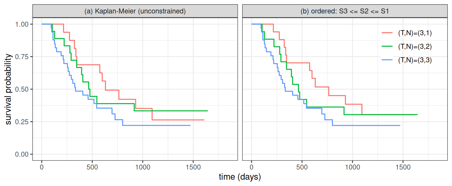
Now the ordering. Take the three T = 3 groups differing in nodal involvement, \((T,N) = (3,1), (3,2), (3,3)\), and impose \(S_3 \preceq S_2 \preceq S_1\) (more nodal involvement, worse survival):
g1 <-list("(3,1)"=grp_counts(3, 1),"(3,2)"=grp_counts(3, 2),"(3,3)"=grp_counts(3, 3))rc_free <-fit_rc(g1)rc_order <-fit_rc(g1, list(c(3, 2), c(2, 1))) # S3 <= S2 <= S1step_rc <-function(fit, groups, panel)do.call(rbind, lapply(seq_along(groups), function(i) { g <- groups[[i]]; S <- fit$S[[i]]; tmax <-attr(g, "tmax") t <-c(0, g$t); s <-c(1, S)if (tmax >max(g$t)) { t <-c(t, tmax); s <-c(s, tail(S, 1)) } # flat KM tail to last obsdata.frame(t = t, S = s,grp =paste0("(T,N)=", names(groups)[i]), panel = panel) }))df <-rbind(step_rc(rc_free, g1, "(a) Kaplan-Meier (unconstrained)"),step_rc(rc_order, g1, "(b) ordered: S3 <= S2 <= S1"))ggplot(df, aes(t, S, colour = grp)) +geom_step(linewidth =0.6) +facet_wrap(~panel) +coord_cartesian(xlim =c(0, 1850), ylim =c(0, 1)) +labs(x ="time (days)", y ="survival probability", colour =NULL) +theme(legend.position ="inside", legend.position.inside =c(0.9, 0.8),legend.background =element_blank())
The unconstrained Kaplan–Meier curves cross — \((3,2)\) sits above \((3,1)\) for much of the range, contradicting \(S_2 \le S_1\) — while the ordered fit removes the crossings, reproducing Figure 1 of Lim et al. (2009). The ordering costs only a little likelihood:
The website’s survival-ordering example carries this further — partial (non-total) orders, a stronger uniform ordering that constrains the hazard ratio, and the interval-censored case, where the same GP recipe applies with a different parameterization.
15.2 Disciplined Quasiconvex Programming (DQCP)
A quasiconvex function has convex sub-level sets but need not be convex itself (think of ratios like \(\|Ax-b\|/c^\top x\)). DCP cannot handle these, but DQCP can, via a sequence of convex feasibility problems; you pass qcp = TRUE. A tiny example minimizes \((a+1)/\sqrt{a}\), which is quasiconvex on \(a > 0\):
a <-Variable(pos =TRUE)prob <-Problem(Minimize((a +1) /sqrt(a)))c(is_dqcp =is_dqcp(prob), optimum =psolve(prob, qcp =TRUE), a =value(a))
  is_dqcp   optimum         a
1.0000000 2.0000000 0.9999228
The minimum is \(2\) at \(a = 1\), found without you having to know the function was quasiconvex. See the DQCP Tutorial.
15.3 Where this leaves us
You now have the whole map: DCP (convex, this book’s backbone), DPP (parametrized, for fast re-solves and derivatives), DGP (log-log convex), DQCP (quasiconvex), and DNLP (smooth nonconvex). Each is the same disciplined bargain — follow the grammar, get a solvable problem — and CVXR checks compliance for you with the matching is_*() predicate. The website’s examples gallery has dozens more worked problems across all of them.
Lim, Johan, Seung Jean Kim, and Xinlei Wang. 2009. “Estimating Stochastically Ordered Survival Functions via Geometric Programming.”Journal of Computational and Graphical Statistics 18 (4): 978–94. https://doi.org/10.1198/jcgs.2009.06140.