10  Sparse Inverse Covariance Estimation

NoteWhat you’ll be able to do

Estimate the graph of conditional dependencies among variables — which ones are related once you account for all the others — by fitting a sparse inverse covariance matrix with a log-determinant objective and an \(\ell_1\) budget.

10.1 The idea

The portfolio chapter (Chapter 9) took a covariance matrix as given. Here we go the other way and estimate it — and specifically its inverse, which carries the more interesting story.

For Gaussian data, the inverse covariance \(S = \Sigma^{-1}\) (the precision matrix) encodes conditional independence: \(S_{ij} = 0\) exactly when variables \(i\) and \(j\) are independent given all the others. So a sparse \(S\) is a sparse graph of direct relationships — often what we actually want to discover. With more variables than the data can pin down, we impose that sparsity directly.

Given i.i.d. samples \(x_i \sim N(0, \Sigma)\) with sample covariance \(Q\), we maximize the Gaussian log-likelihood while capping the total size of \(S\):

\[ \begin{array}{ll} \underset{S}{\mbox{maximize}} & \log\det(S) - \mathop{\mathrm{tr}}(SQ) \\ \mbox{subject to} & S \succeq 0, \qquad \sum_{i,j} |S_{ij}| \le \alpha . \end{array} \]

The \(\ell_1\) budget \(\alpha \ge 0\) controls sparsity: smaller \(\alpha\) forces more off-diagonal entries to exactly zero. The objective is concave (log_det is concave; the trace term is linear) and the constraints are convex, so CVXR solves it directly.

10.2 Synthetic data with a known answer

So we can check the estimate, we build a true sparse precision matrix \(S_{\text{true}}\), invert it to get the covariance \(R\), and sample from \(N(0, R)\):

set.seed(1)
n <- 10        # number of variables
m <- 1000      # number of samples

A      <- rsparsematrix(n, n, 0.15, rand.x = rnorm)
Strue  <- as.matrix(A %*% t(A) + 0.05 * diag(n))   # sparse, symmetric, positive definite
R      <- solve(Strue)                              # the covariance to sample from

x <- matrix(rnorm(m * n), m, n) %*% chol(R)         # rows are i.i.d. N(0, R)
Q <- cov(x)                                          # sample covariance

sum(abs(Strue) > 1e-4)                               # how many true nonzeros (of 100)

[1] 24

10.3 Fit at several sparsity budgets

A semidefinite variable is declared with PSD = TRUE. We sweep \(\alpha\) and, after each solve, zero out numerically negligible entries to read off the recovered pattern:

alphas <- c(10, 6, 4, 1)
S      <- Variable(c(n, n), PSD = TRUE)
obj    <- Maximize(log_det(S) - matrix_trace(S %*% Q))

S_est <- lapply(alphas, function(a) {
  prob <- Problem(obj, list(sum(abs(S)) <= a))
  psolve(prob)
  check_solver_status(prob)
  Sa <- value(S)
  Sa[abs(Sa) <= 1e-4] <- 0            # treat tiny entries as exact zeros
  Sa
})
sapply(S_est, function(M) sum(M != 0))  # nonzeros recovered at each alpha

[1] 46 32 24 12

Note matrix_trace(S %*% Q) rather than sum(diag(S %*% Q)) — same value, but the dedicated atom keeps the expression tree compact. And log_det(S) is its own atom: there is no det() for a CVXR variable, because the log-determinant is the convex object DCP understands.

10.4 What the budget buys

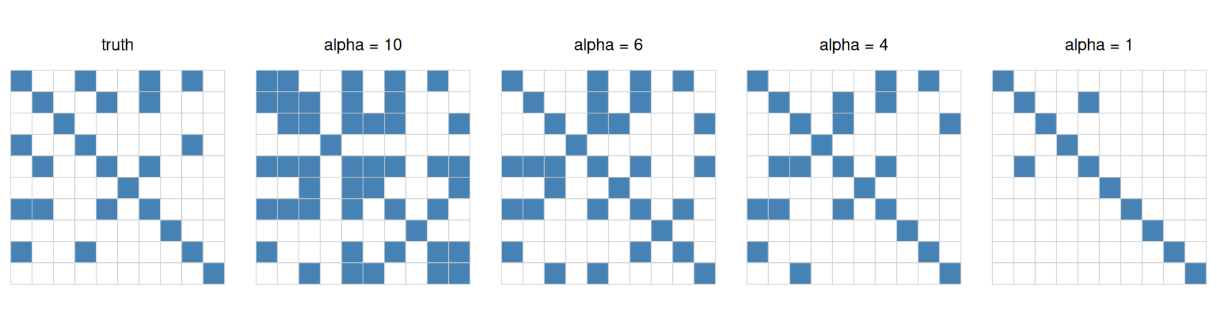
The sparsity pattern of the estimate tightens as \(\alpha\) shrinks. We plot the nonzero mask of the truth alongside each fit:

mask_df <- function(M, lab) {
  data.frame(i = rep(seq_len(n), n), j = rep(seq_len(n), each = n),
             nz = factor(as.integer(as.vector(M) != 0)), panel = lab)
}
panels <- rbind(
  mask_df(Strue, "truth"),
  do.call(rbind, Map(function(M, a) mask_df(M, paste0("alpha = ", a)), S_est, alphas)))
panels$panel <- factor(panels$panel, levels = c("truth", paste0("alpha = ", alphas)))

ggplot(panels, aes(i, j, fill = nz)) +
  geom_tile(color = "grey80") +
  scale_fill_manual(values = c("0" = "white", "1" = "steelblue"), guide = "none") +
  scale_y_reverse() + coord_equal() +
  facet_wrap(~ panel, nrow = 1) +
  theme_void() + theme(strip.text = element_text(margin = margin(4, 0, 4, 0)))

Nonzero pattern (dark = nonzero) of the true precision matrix and the estimates. Smaller alpha -> sparser. Around alpha = 4 the estimate matches the truth’s sparsity.

At \(\alpha = 10\) the budget is loose and the estimate is dense; as \(\alpha\) falls the off-diagonal entries are squeezed to zero, and near \(\alpha = 4\) the recovered pattern matches the true number of nonzeros. Too small (\(\alpha = 1\)) and we lose real edges. In practice you would pick \(\alpha\) by cross-validation — and because the only thing changing across the sweep is one constant, this is a textbook case for the Parameter trick of Chapter 8.

10.5 Takeaways

• The inverse covariance is the object of interest: its zeros are conditional independencies — a graph of direct relationships.
• log_det(S) - matrix_trace(S %*% Q) with S declared PSD = TRUE and an \(\ell_1\) budget is the whole model — a few lines of CVXR.
• One knob, \(\alpha\), trades density for sparsity; sweep it with a Parameter.

See Sparse Inverse Covariance Estimation for the full treatment.