12  Image Reconstruction

NoteWhat you’ll be able to do

Reconstruct a corrupted image by total-variation in-painting — a convex model that fills in missing pixels with no machine-learning training, just “match what you know and stay smooth.”

12.1 Repairing a damaged image

A grayscale image is just a matrix of pixel intensities. Suppose some pixels are corrupted (here, white text scrawled over the picture) and we know which ones. Can we fill them in? The total-variation in-painting model says: among all images that agree with the known pixels, choose the one with the smallest total variation — the least “jumpy” one. Total variation of \(U\) is

\[\mathop{\mathbf{tv}}(U) = \sum_{i,j}\left\|\begin{pmatrix} U_{i+1,j}-U_{ij}\\ U_{i,j+1}-U_{ij}\end{pmatrix}\right\|_2,\]

a convex function, so the whole problem is convex. We load a \(128\times128\) image and a corrupted copy, and mark a pixel known where the two agree:

u_orig <- readPNG("images/loki128.png")
u_corr <- readPNG("images/loki128_corrupted.png")
if (length(dim(u_orig)) == 3) u_orig <- (u_orig[,,1] + u_orig[,,2] + u_orig[,,3]) / 3
if (length(dim(u_corr)) == 3) u_corr <- (u_corr[,,1] + u_corr[,,2] + u_corr[,,3]) / 3
rows <- nrow(u_orig); cols <- ncol(u_orig)
known <- 1 * (u_orig == u_corr)        # 1 where the pixel survived
cat(sprintf("%d x %d image; %.0f%% of pixels known\n",
            rows, cols, 100 * sum(known) / (rows * cols)))

128 x 128 image; 86% of pixels known

The model is a direct transcription of the math: minimize total variation subject to matching the known pixels.

U <- Variable(c(rows, cols))
prob <- Problem(Minimize(total_variation(U)),
                list(known * U == known * u_corr))
psolve(prob, solver = "SCS")          # ~16k variables; a few seconds

[1] 740.1374

U_val <- pmin(pmax(value(U), 0), 1)   # clip to [0, 1]
cat("status:", status(prob), "\n")

status: optimal 

show_img <- function(m, title) {
  plot(c(0, 1), c(0, 1), type = "n", axes = FALSE, xlab = "", ylab = "",
       main = title, asp = 1)
  rasterImage(as.raster(m), 0, 0, 1, 1, interpolate = FALSE)
}
op <- par(mfrow = c(1, 3), mar = c(1, 1, 2, 1))
show_img(u_orig, "Original")
show_img(u_corr, "Corrupted")
show_img(U_val,  "In-painted")

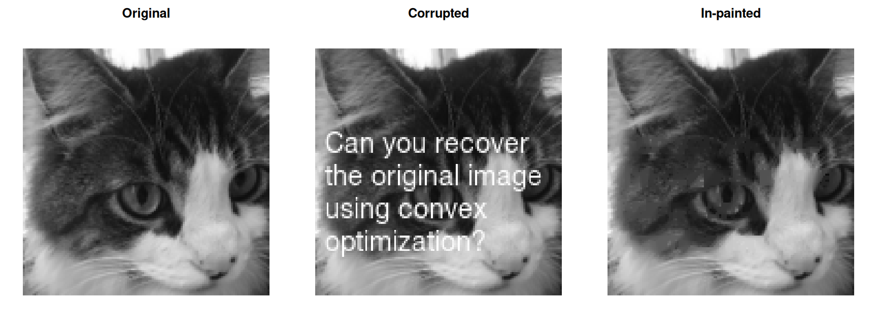
Original, corrupted, and in-painted (the text is gone).

par(op)

The solver never “knew” it was looking at a face — it just found the smoothest image consistent with the surviving pixels. That is the power of a good convex model.

12.2 Takeaways

• A convex model (total variation) reconstructs a damaged image with no machine-learning training — just “match the known pixels, stay smooth.”
• The unknowns are the ~16,000 pixels of an entire image, yet the model is three lines of CVXR; the structure lives in the objective, not in bespoke code.
• The same in-painting idea extends to denoising, deblurring, and compressed sensing — swap the data-fit term, keep the smoothness penalty.

See TV In-Painting for color images and more variants.